Introduction
Julia is a general purpose programming language, used for numerical analysis and scientific computing.
It uses JIT compiler to execute code for faster computational speed. It allows Multiple dispatch which means all of it's
functional arguments to choose which method should be invoked at a given time.
Some other key points:
- Julia's indexing is one-based and ranges are inclusive instead of exclusive
- Julia is functional programming language not object orientated like python
Getting started
Installation
Linux users can install Julia using their native package manager. For Windows and macOS, head to the official website https://julialang.org/downloads/ to download the specific version and install it into your system. Ensure that Julia is in the system path and accessible from terminal/cmd (to check: $ julia --version).
Julia has built-in REPL and interactive session can be invoked by typing julia on the terminal
❯ julia
_
_ _ __ | Documentation: https://docs.julialang.org
| |
_ _ _| |_ __ _ | Type for help, for Pkg help.
| | | | | | |/ _Hello, World!
Since you have installed Julia in your system and now the time is write the first hello world program.
The file extension of Julia is .jl and code can be directly executed as
# FILE: helloworld.jl
println("Hello, World!")
Add a package
press ] in Julia interactive session to switch package manager mode
add IJulia
to get back the terminal press Backspace
or package can be install from Julia REPL
using Pkg
Pkg.add
IJulia is a Jupyter kernel for interactive jupyter environment like IPython (interactive python)
to write code inside jupyter notebook
Pluto (add Pluto) on the otherhand reactive and lightweight notebook written in Julia.
Start the Pluto server
julia> import Pluto
julia> Pluto.run
Some Scientific Packages to consider
Distributions  <-- Statistics
DifferentialEquations  <-- DE solve
Plots  <-- Plotting
Programming Concepts
Julia Lang shares the same programming concepts similar to other programming languages such as Python, C.
Numbers and Operators
julia> # Addition of two integer
julia> 1 + 2
3
julia> # Substraction
julia> 20 - 2.2
17.8
julia> # Modulo division
julia> 21//20
21//20
julia> # Multiplication
julia> 5 * pi
15.707963267948966
julia> x =
"Julia"
julia> typeof
String
String
julia> name =
"Sanatan"
julia> name
: /Unicode U+006E
julia> for letter in name
println
end
S
a
n
a
t
a
n
Array
julia> x =
3-element Vector{Int64}:
1
2
3
julia> x # should give error because of one-based index
ERROR: BoundsError: attempt to access 3-element Vector{Int64} at index
Stacktrace:
getindex
@ Base ./essentials.jl:13
top-level scope
@ REPL:1
julia> x
1
julia> x # ranges are inclusive means elements at index 3 is included
3-element Vector{Int64}:
1
2
3
julia> y = ' # column vector
1×3 adjoint with eltype Int64:
1 2 3
julia> xl = range # linspace function
1.0:0.4444444444444444:5.0
julia> xz = zeros # 2x2 matrix with all elements as zeros
2×2 Matrix{Float64}:
0.0 0.0
0.0 0.0
Function
julia>
f function returns the value of last expression, but also function can return at any point
julia>
g for the function g, a + b is never executed so thisl ine is poitnless, we can just write a * b at the last without return keyword. return is helpful when some condition is applied
Control flow
if-else
julia>
h looping
julia> for i=1:10
println
end
1
2
3
4
5
6
7
8
9
10
Plot
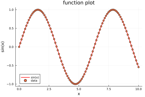
Plots package provide nice and rich graphics library for plotting scientific data. Here a simple example
for basic 2d plot
using Plots
x = range
y = sin.
plot
plot!
xlabel!
ylabel!
savefig
